Neural Network From Scratch With NumPy
Neural networks often feel like magic—high-level libraries abstract away the math, GPUs crunch the numbers, and with a few lines of code, models start making predictions. But beneath the convenience of frameworks like TensorFlow and PyTorch lies a beautifully simple set of mathematical operations. In this blog, we’ll strip away the abstractions and build a neural network from scratch using nothing but NumPy.
We will understand how training and backpropagation works under the hood. TLDR; The notebook implementation of this blog is available here.
What do we want our model to predict?
For this implementation, we’ll train our neural network to classify handwritten digits from the famous MNIST dataset.
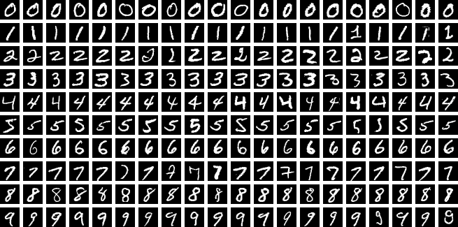
Source: https://en.wikipedia.org/wiki/MNIST_database
Download and Prepare Dataset
We can use scikit-learn to make things easier here. Install the library in your virtual environment. Loading MNIST with scikit-learn is just oneliner and it directly gives us images as NumPy array.
pip install scikit-learn
Load the dataset with the following code snippet:
import sklearn

X, y = sklearn.datasets.fetch_openml("mnist_784", return_X_y=True, as_frame=False)
print(X.shape, y.shape)
(70000, 784) (70000,)
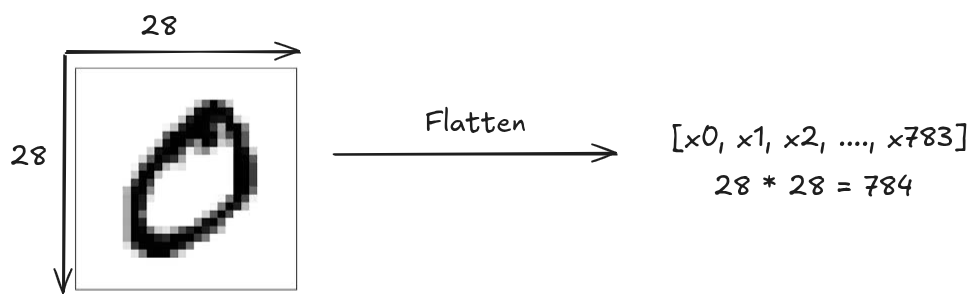
As you can see there are 70,000 images with feature size of 784 and their corresponding target labels. The MNIST dataset contains 70,000 grayscale images of 28x28 pixels hand written digits (0 to 9). Each image is flattened into a vector of 784 features.
Pre-processing the dataset
Lets observe the first input image of the dataset.
import matplotlib.pyplot as plt

plt.imshow(X[0].reshape(28, 28), cmap="gray")

print(X[0])
[  0   0   0   0   0   0   0   0   0   0   0   0   0   0   0   0   0   0
   0   0   0   0   0   0   0   0   0   0   0   0   0   0   0   0   0   0
   0   0   0   0   0   0   0   0   0   0   0   0   0   0   0   0   0   0
   0   0   0   0   0   0   0   0   0   0   0   0   0   0   0   0   0   0
   0   0   0   0   0   0   0   0   0   0   0   0   0   0   0   0   0   0
   0   0   0   0   0   0   0   0   0   0   0   0   0   0   0   0   0   0
   0   0   0   0   0   0   0   0   0   0   0   0   0   0   0   0   0   0
   0   0   0   0   0   0   0   0   0   0   0   0   0   0   0   0   0   0
   0   0   0   0   0   0   0   0   3  18  18  18 126 136 175  26 166 255
 247 127   0   0   0   0   0   0   0   0   0   0   0   0  30  36  94 154
 170 253 253 253 253 253 225 172 253 242 195  64   0   0   0   0   0   0
   0   0   0   0   0  49 238 253 253 253 253 253 253 253 253 251  93  82
  82  56  39   0   0   0   0   0   0   0   0   0   0   0   0  18 219 253
 253 253 253 253 198 182 247 241   0   0   0   0   0   0   0   0   0   0
   0   0   0   0   0   0   0   0  80 156 107 253 253 205  11   0  43 154
   0   0   0   0   0   0   0   0   0   0   0   0   0   0   0   0   0   0
   0  14   1 154 253  90   0   0   0   0   0   0   0   0   0   0   0   0
   0   0   0   0   0   0   0   0   0   0   0   0   0 139 253 190   2   0
   0   0   0   0   0   0   0   0   0   0   0   0   0   0   0   0   0   0
   0   0   0   0   0  11 190 253  70   0   0   0   0   0   0   0   0   0
   0   0   0   0   0   0   0   0   0   0   0   0   0   0   0   0  35 241
 225 160 108   1   0   0   0   0   0   0   0   0   0   0   0   0   0   0
   0   0   0   0   0   0   0   0   0  81 240 253 253 119  25   0   0   0
   0   0   0   0   0   0   0   0   0   0   0   0   0   0   0   0   0   0
   0   0  45 186 253 253 150  27   0   0   0   0   0   0   0   0   0   0
   0   0   0   0   0   0   0   0   0   0   0   0   0  16  93 252 253 187
   0   0   0   0   0   0   0   0   0   0   0   0   0   0   0   0   0   0
   0   0   0   0   0   0   0 249 253 249  64   0   0   0   0   0   0   0
   0   0   0   0   0   0   0   0   0   0   0   0   0   0  46 130 183 253
 253 207   2   0   0   0   0   0   0   0   0   0   0   0   0   0   0   0
   0   0   0   0  39 148 229 253 253 253 250 182   0   0   0   0   0   0
   0   0   0   0   0   0   0   0   0   0   0   0  24 114 221 253 253 253
 253 201  78   0   0   0   0   0   0   0   0   0   0   0   0   0   0   0
   0   0  23  66 213 253 253 253 253 198  81   2   0   0   0   0   0   0
   0   0   0   0   0   0   0   0   0   0  18 171 219 253 253 253 253 195
  80   9   0   0   0   0   0   0   0   0   0   0   0   0   0   0   0   0
  55 172 226 253 253 253 253 244 133  11   0   0   0   0   0   0   0   0
   0   0   0   0   0   0   0   0   0   0 136 253 253 253 212 135 132  16
   0   0   0   0   0   0   0   0   0   0   0   0   0   0   0   0   0   0
   0   0   0   0   0   0   0   0   0   0   0   0   0   0   0   0   0   0
   0   0   0   0   0   0   0   0   0   0   0   0   0   0   0   0   0   0
   0   0   0   0   0   0   0   0   0   0   0   0   0   0   0   0   0   0
   0   0   0   0   0   0   0   0   0   0   0   0   0   0   0   0   0   0
   0   0   0   0   0   0   0   0   0   0]
As we can clearly see that the pixel values are in range between 0 and 255. We should normalize this range to 0 and 1. Normalizing has lots of advantage in machine learning, it helps improve numerical stability, prevents feature dominance and speeds up the training time.
X = X / 255.0
Similarly, looking at the target label of this first image.
print(y[0])
'5'
OpenML stores categorical data as strings. It would be
easier to process numeric target instead of strings. So, we convert data type of
target y to numeric.
import numpy as np

y = y.astype(np.int64)
We must perform an another important pre-processing step for target label y as well.
Currently, the target label are as [5, 0, 4, 9, .....]. We want to perform one-hot
encoding of this categorical data into a numerical binary format.
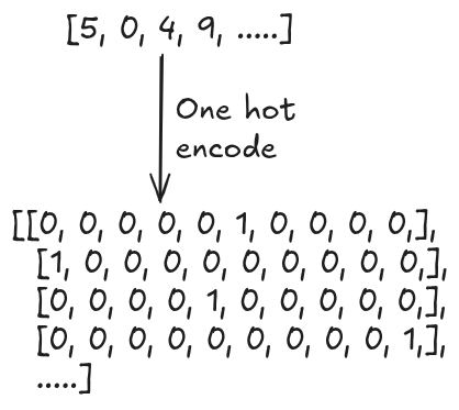
def one_hot(y):
    out = np.zeros((y.size, y.max().item() + 1))
    out[np.arange(y.size), y] = 1
    return out
We one-hot encode all the target labels:
Y = one_hot(y)
Finally, we will split 80% of dataset for training and rest 20% for evaluating the model. We also keeping non encoded target label which will be required during evaluation.
from sklearn.model_selection import train_test_split

X_train, X_test, Y_train, Y_test, y_train, y_test = train_test_split(X, Y, y, test_size=0.2)
Fully Connected Neural Network
We’ll build a simple 2-layer neural network.
Input (784)
    ↓
Hidden Layer (128 neurons, ReLU)
    ↓
Output Layer (10 neurons, Softmax)
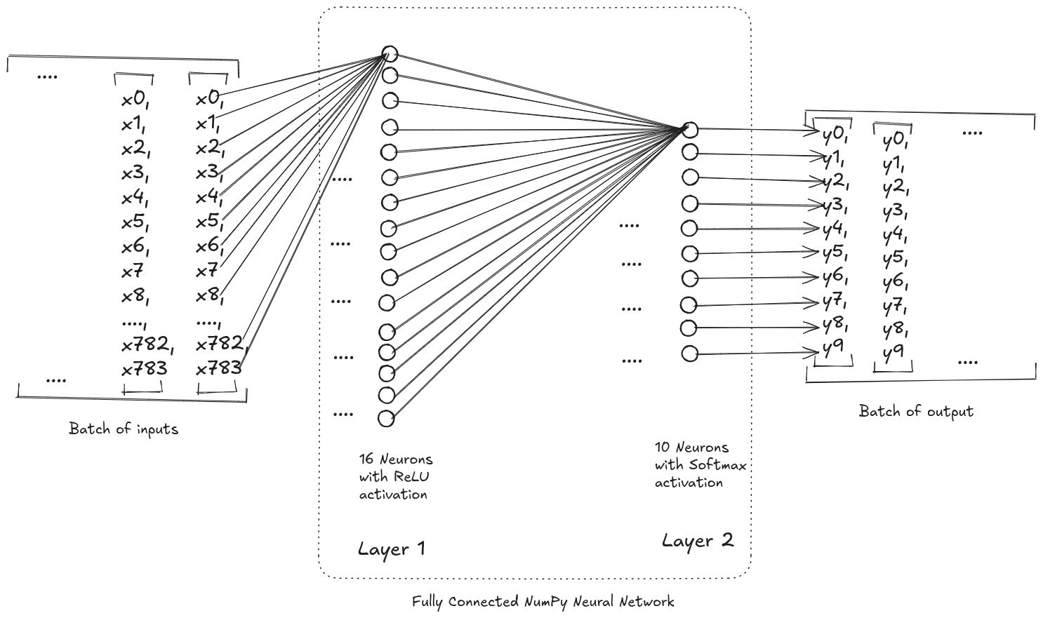
This is a fully connected (dense) feedforward network.
Data Flow in the network
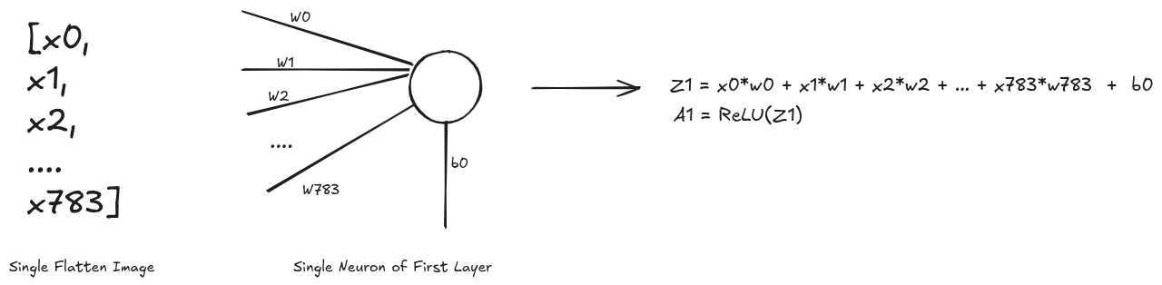
For first layer, talking one example input image and a neuron, we obtain a1
as the output. The operation performed on batch of input array and all the neurons of
the first layer to yield z1 is simply the matrix multiplication @. After which we
perform the ReLU activation
function which is fairly simple to implement. Due to this matrix operation you might
see transpose operation <array>.T being performed in order to obtain the required
output else where in the code.
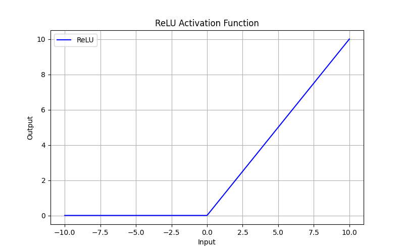
def ReLU(z):
    return np.maximum(0, z)
We will be needing the derivative of ReLU function during the backpropagation so lets take a look its implementation and plot as well.
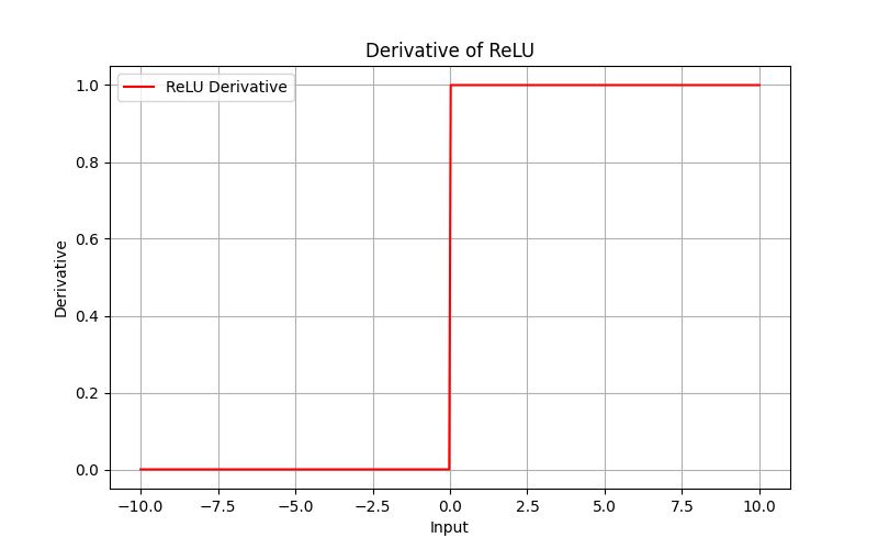
def ReLU_deriv(z):
    return (z > 0).astype(np.float64)
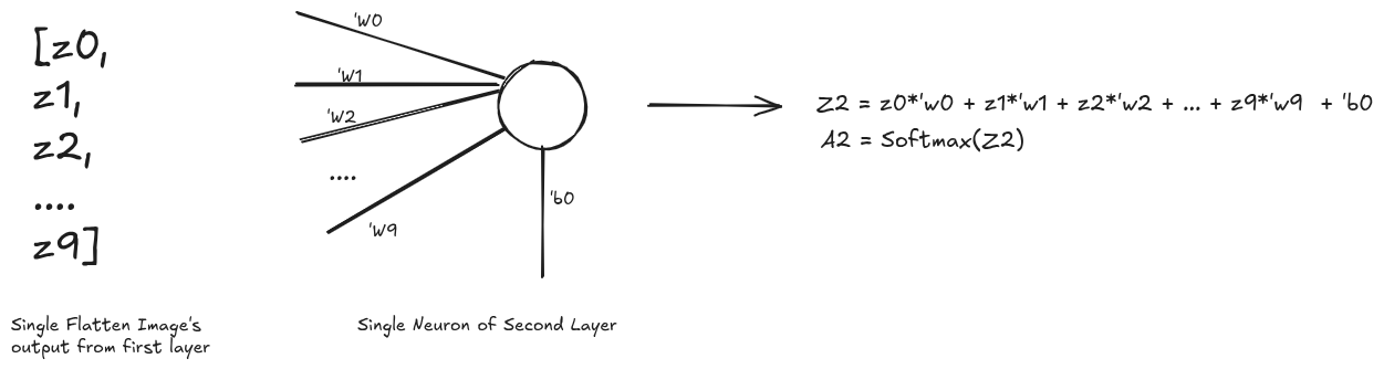
Similarly, taking the single output from first layer into the second layer is almost the same expect for the activation function. In the second layer we will be using Softmax function.
[WIP]…